Model Coding:

Created: June 18, 2025 6:09 PM Tags: article note

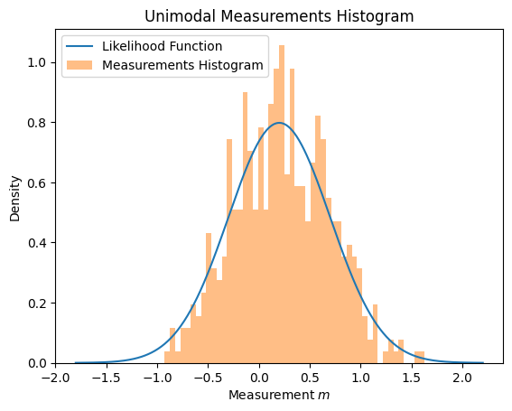
1- Unimodal

1.1 Measurement

imageHo

\[m=N(s,\sigma^2)\]

# unimodal measurements
def unimodalMeasurements(sigma, S):
    # P(x|s) # generate measurements from a normal distribution
    m = np.random.normal(S, sigma**2, 10000)  # true duration is S seconds
    return m

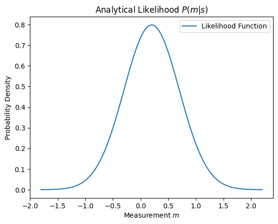
1.2 Likelihood

\[p(m|s)=\frac{1}{\sqrt{2\pi} \sigma}\exp(-\frac{(m-s)^2}{2\sigma^2})\]

def gaussianPDF(m,s,sigma):
    return (1/(np.sqrt(2*np.pi)*sigma))*np.exp(-((x-s)**2)/(2*(sigma**2)))

# likelihood function
def likelihood(S, sigma):
    # P(m|s) # likelihood of measurements given the true duration
    m=np.linspace(S - 4*sigma, S + 4*sigma, 500)
    p_x=gaussianPDF(m,S,sigma)
    return x, p_x

1.2.1 Plot Likelihoods analytically

def plotLikelihood(S,sigma):
    x, p_x = likelihood(S, sigma)
    plt.plot(x, p_x, label='Likelihood Function')
    plt.xlabel('Measurement $m$')
    plt.ylabel('Probability Density')
    plt.title('Analytical Likelihood $P(m|s)$')
    plt.legend()
    
def plotMeasurements(sigma, S):
    m = unimodalMeasurements(sigma, S)
    plt.hist(m, bins=50, density=True, alpha=0.5, label='Measurements Histogram')
    plt.xlabel('Measurement $m$')
    plt.ylabel('Density')
    plt.title('Unimodal Measurements Histogram')
    plt.legend()      

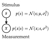
2 Bimodal

graph TD
  A(C) --> B1(C=1)
  A --> b2(C=2)
  B1-->b11(S)
  b11-->b111(m_a)
  b11-->b112(m_v)
  b2-->b21(S_a)
  b2-->b22(S_v)
  b21-->b211(m_a)
  b22-->b212(m_v)

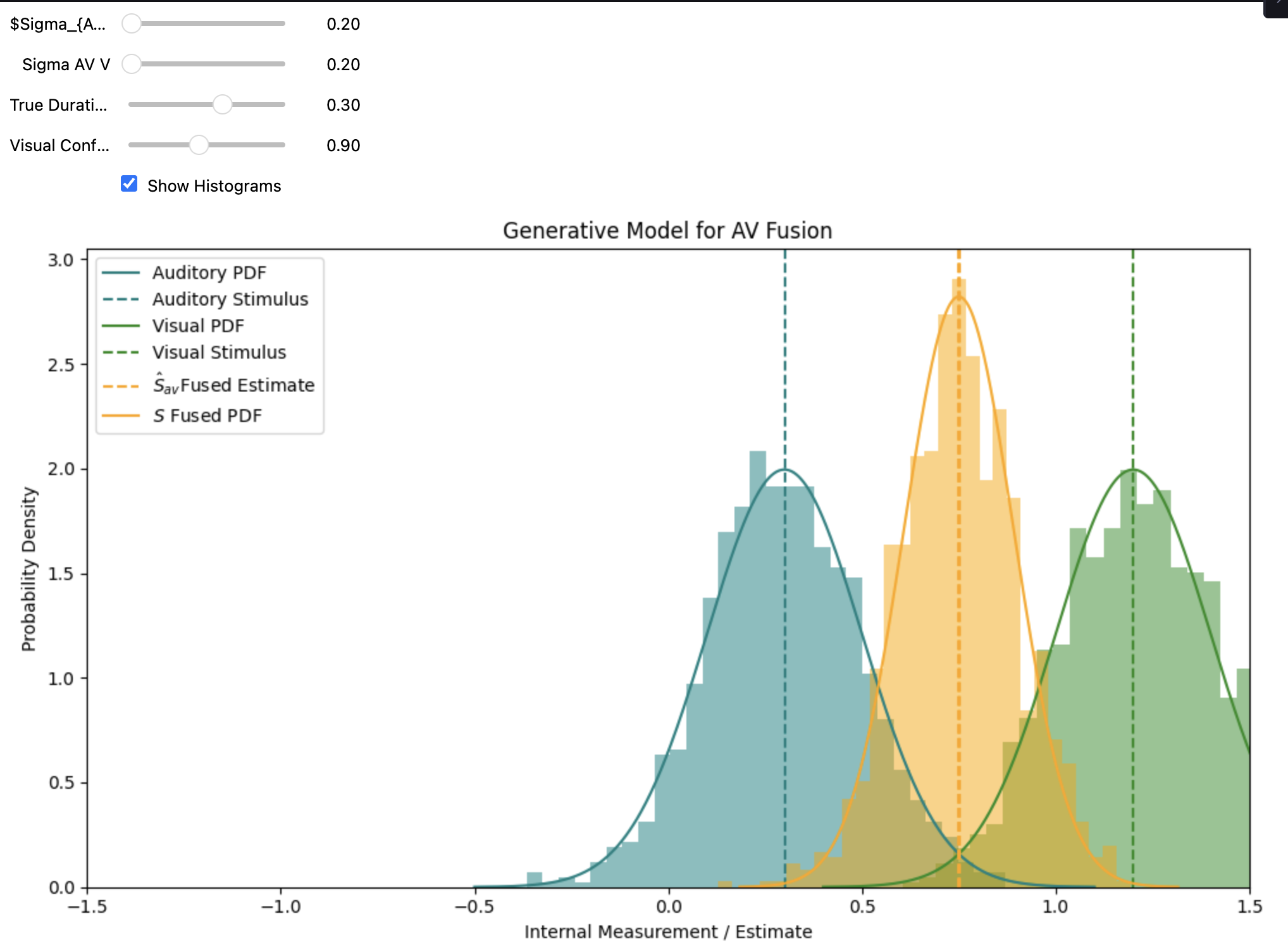
2.1 Fusion (C=1)

2.1.1 Fusion of one interval

\[\hat{S}_{av,a}=\hat{S}_{av,v}= \frac{\sigma_{av,a}^{-2} m_a+\sigma_{av,v}^{-2} m_v}{\sigma_{av,a}^{-2} + \sigma_{av,v}^{-2}}\\ = w_aS_a+w_vS_v\] \[J_a=\frac{1}{\sigma_{av,a}^{2}} \\ J_v=\frac{1}{\sigma_{av,v}^{2}}\\ \sigma_{av}^2=\frac{1}{J_1+J_2}\] \[p(S|m_a,m_v)\sim p(S)p(m_a|S)p(m_v|S)\\\] \[p(S|m_a,m_v)\sim N(\hat S_{av},\sigma_{av}^2)\\\] \[p(S|m_a,m_v)= \frac{1}{\sqrt{2\pi} \sigma_{av}}\exp(-\frac{(S-\hat S_{av})^2}{2\sigma_{av}^2})\]

def fusionAV(sigmaAV_A,sigmaAV_V, S_a, visualConflict):
    m_a=unimodalMeasurements(sigmaAV_A, S_a)
    S_v=S_a+visualConflict
  m_v = unimodalMeasurements(sigmaAV_V,S_v )  # visual measurement
  # compute the precisons inverse of variances
  J_AV_A= sigmaAV_A**-2 # auditory precision
  J_AV_V=sigmaAV_V**-2 # visual precision
  # compute the fused estimate using reliability weighted averaging
  hat_S_AV= (J_AV_A*m_a+J_AV_V*m_v)/(J_AV_V+J_AV_A)
    mu_Shat = w_a * S_a + w_v * S_v  # fused mean
  sigma_S_AV_hat = np.sqrt(1 / (J_a + J_v))  # fused standard deviation

  return hat_S_AV , sigma_S_AV_hat # belief about fused stimulus value

2.1.2 Fusion of 2-IFC Duration Difference

$\Delta_{t-s}$ is the duration difference between t (test interval) and s (standard interval)

$m_{a,t}$ = measurement for auditory test duration.

$m_{a,t}$ = measurement for auditory standard duration.

$c$ = conflict duration incorporated to the visual standard stimulus.

\[\Delta_{t-s}=w_a({m_{a,t}} -m_{a,s})+ w_v ({m_{v,t}} -m_{v,s})\\=w_a\Delta S_a +w_v \Delta S_v\] \[m_{a,t} - m_{a,s} \sim N(\Delta s_a, 2\sigma^2_a)\\ m_{v,t} - m_{v,s} \sim N(\Delta s_v, 2\sigma^2_v)\]

The difference between two interval within single trial:

\[\Delta_{t-s} = w_a(m_{a,t} - m_{a,s}) + w_v(m_{v,t} - (m_{v,s}))\\ \sim N(w_a\Delta s_a + w_v\Delta s_v, 2\sigma^2_{av})\] \[\Delta_{t-s} \sim N(\hat S_t - \hat S_s,2\sigma_{av}^2)\]

Expected value of duration difference

Test Interval:

\[E[m_{v,t}]=E[m_{a,t}]=S_{v,t}=S_{a,t}\]

Standard interval:

\[E[m_{a,s}]=S_{v,s}=S_{a,s}+c\]

Duration difference:

\[E[\Delta_{t-s}] = w_a(s_{a,t} - s_{a,s}) + w_v(s_{v,t} - s_{v,s})\]

substituting:

\[S_{v,s}=S_{a,s}+c\] \[\begin{aligned} E[\Delta_{t-s}] &= w_a(s_{a,t} - s_{a,s}) + w_v[s_{a,t} - (s_{a,s} + c)] \\ &= w_a(s_{a,t} - s_{a,s}) + w_v(s_{a,t} - s_{a,s} - c) \\ &= (w_a + w_v)(s_{a,t} - s_{a,s}) - w_v c \\ &= (s_{a,t} - s_{a,s}) - w_v c \end{aligned}\]

Notice that sum of weights equal to 1 as we assume fusion.

Final predict:

\[\Delta_{t-s}=N((S_{a,t}-S_{a,s})-w_vc,2\sigma_{av}^2)\]

$w_vc$ is predicted bias:

if c>0 standard visual is longer), the standard is perceived as longer, so test needs to be even longer to be matched.
The PSE shifts by $w_vc$

Decision Rule:

\[P(\text{"test longer"}) = \Phi\left(\frac{(S_{a,t} - S_{a,s}) - w_v c}{\sqrt{2}\sigma_{av}}\right)\]

2.2 Causal inference of 2-IFC Duration Difference ( C=1 , C=2)

2.2.1 No common cause (C=2)

In the case of no common cause, the observer infers that the auditory and visual durations are independent, so that the posterior estimate of different modalities are independent as well.

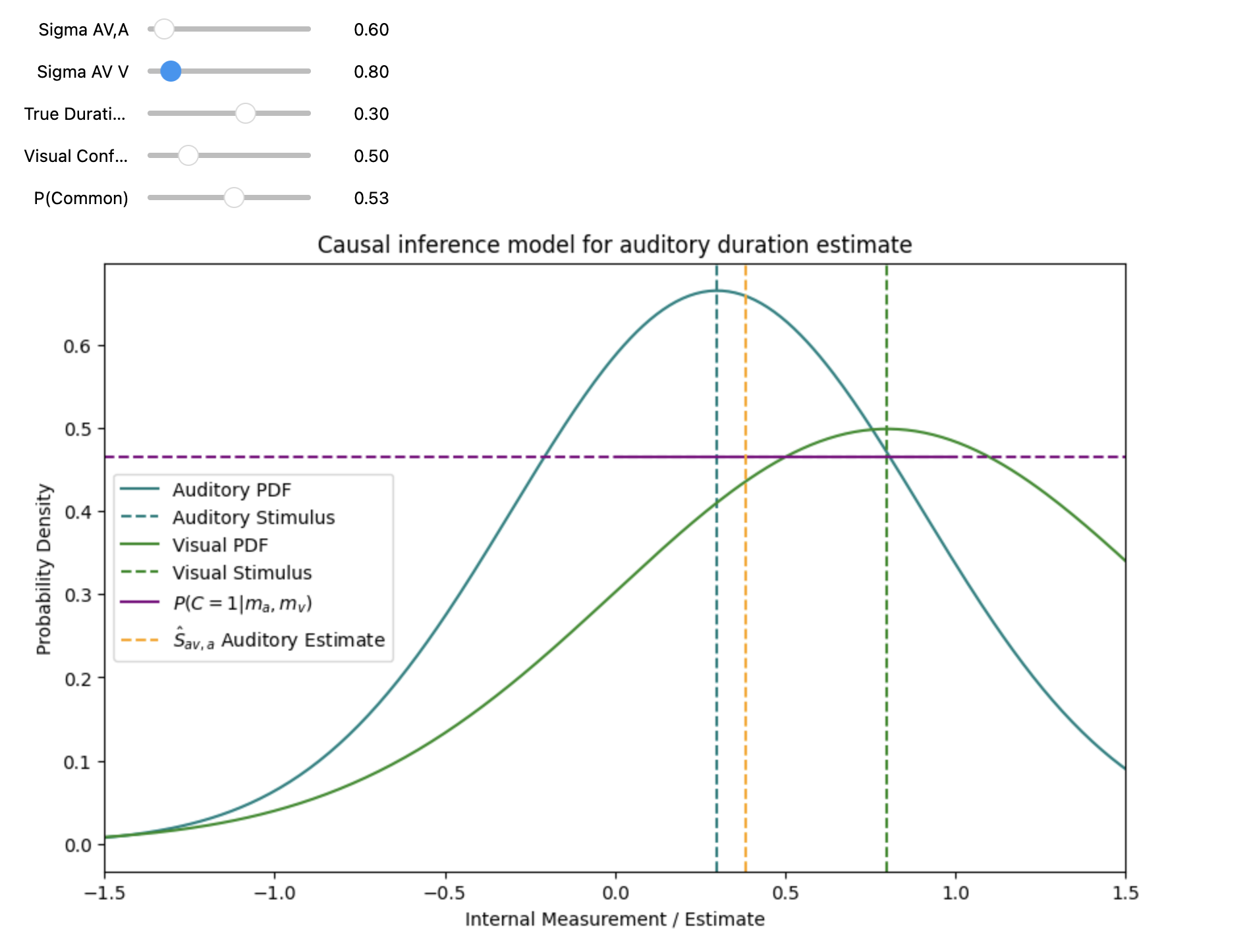
\[\hat S_{av,a}= m_a, \hat S_{av,v}= m_v, \\ \sigma_{av,a}^2=\sigma_a^2, \sigma_{av,v}^2=\sigma_v^2,\]

We assume that common cause inference is not a binary decision, but rather a continuous variable that can take any value between 0 and 1. The observer can then use this variable to weight the auditory and visual durations in their final estimate. The final estimate is given by:

\[\hat S_{av,a}= \hat S_{av,a} \cdot P(C=1|m_a, m_v) + \hat S_{av,a} \cdot (1 - P(C=1|m_a, m_v))\]

Where $P(C=1

S_a, S_v)$ is the posterior probability of the common cause given the auditory and visual durations. Observer has measurements:

\[\text{Auditory measurement}= m_a\\ \text{Visual measurement}= m_v\\\]

Each is noisy sample:

\[m_a \sim N(S_a, \sigma_{av,a}^2)\\ m_v\sim N(S_v, \sigma_{av,v}^2)\\\]

Here, measurement noise $\sigma_{av,a}$ and $\sigma_{av,v}$ is fit directly from AV bimodal experiment data; we do not assume they are identical to unimodal noise( $\sigma_{av,a} \ne \sigma_a$) as the variance should depend on the context.

This model allows the observer to flexibly integrate the auditory and visual durations based on their prior beliefs about the common cause, leading to more accurate estimates of the durations.

Similarly for the visual duration estimate would be:

\[\hat S_{av,v}= \hat S_{av,v} \cdot P(C=1|m_a, m_v) + \hat S_{av,v} \cdot (1 - P(C=1|m_a, m_v))\]

At this point to solve the model we need to obtain the probability of common source.

\[P(C|m_a,m_v)=\frac{P(m_a,m_v|C)P(C)}{P(m_a,m_v)}\]

and in this case $p(c=1|m_a,m_v)+p(c=2|m_a,m_v)=1$ When we expand the the common source equation for $C=1$ posterior would be:

Final percept:

\[P(C=1|m_a,m_v)=\frac{p(m_a,m_v|C=1)\cdot p(C=1)}{p(m_a,m_v|C=1)p(C=1)+p(m_a,m_v|C=2)(1-p(c=1))}\] \[\text{Final auditory estimate}=P(C=1|m_a, m_v)\cdot Fused+ (1-P(C=1|m_a, m_v))\cdot\text{Auditory Only}\]

Simply the decision would be:

\[P(\text{“test longer”}) = \Phi\left(\frac{\hat{S}_{\text{final},t} - \hat{S}_{\text{final},s}}{\sqrt{2}\,\sigma_{\text{decision}}}\right)\]

And the posterior probability for not a common source is: $1-P(C=1

m_a,m_v)$

Now the problem becomes how to estimate the likelihood of the common source given the auditory and visual measurements.

The likelihood of the common source can be estimated using a Gaussian distribution, assuming that the auditory and visual measurements are independent given the common cause. The likelihood can be expressed as:

\[p(m_a,m_v|C=1)= \int p(m_a,m_v|s_{a,v}) p(s_{a,v}) d_{s_{a,v}}\\ = \int p(m_a|s_{a,v})p(m_v|s_{a,v}) p(s_{a,v}) d_{s_{a,v}}\\\]

Likelihood of the common cause (C=1):

Compute:

\[P(m_a,m_v|C=1)\] \[P(m_a, m_v | C=1) =\frac{1}{2\pi\sqrt{\sigma_{av,a}^2 \sigma_{av,v}^2+ \sigma_{av,a}^2 \sigma_p^2+ \sigma_{av,v}^2 \sigma_p^2}}\times\ \exp \left(- \frac{1}{2}\frac{(m_a - m_v)^2 \sigma_p^2+ (m_a - \mu_p)^2 \sigma_{av,v}^2+ (m_v - \mu_p)^2 \sigma_{av,a}^2}{\sigma_{av,a}^2\sigma_{av,v}^2 + \sigma_{av,a}^2\sigma_p^2 + \sigma_{av,v}^2\sigma_p^2}\right)\] \[P(m_a, m_v \mid C = 1) = \frac{1}{\sqrt{2\pi(\sigma^2_{a} + \sigma^2_{v})}} \exp\left(-\frac{(m_a - m_v)^2}{2(\sigma^2_{a} + \sigma^2_{v})}\right)\]

Derivation of final likelihood formula

Detailed derivation of integrand:

Combine terms by s

\[p(m_1, m_2 \mid C = 1) =\frac{1}{(2\pi)^{3/2} \sigma_a \sigma_v \sigma_p} \exp\left( - \frac{m_a^2}{2\sigma_a^2} - \frac{m_v^2}{2\sigma_v^2} - \frac{\mu_p^2}{2\sigma_p^2}\right)\int \exp\left( -\frac{A s^2 - 2Bs}{2} \right) ds\]

Where:

\[A = \frac{1}{\sigma_a^2} + \frac{1}{\sigma_v^2} + \frac{1}{\sigma_p^2}, \quad B = \frac{m_a}{\sigma_a^2} + \frac{m_v}{\sigma_v^2} + \frac{\mu_p}{\sigma_p^2}\]

Here we try to complete the square

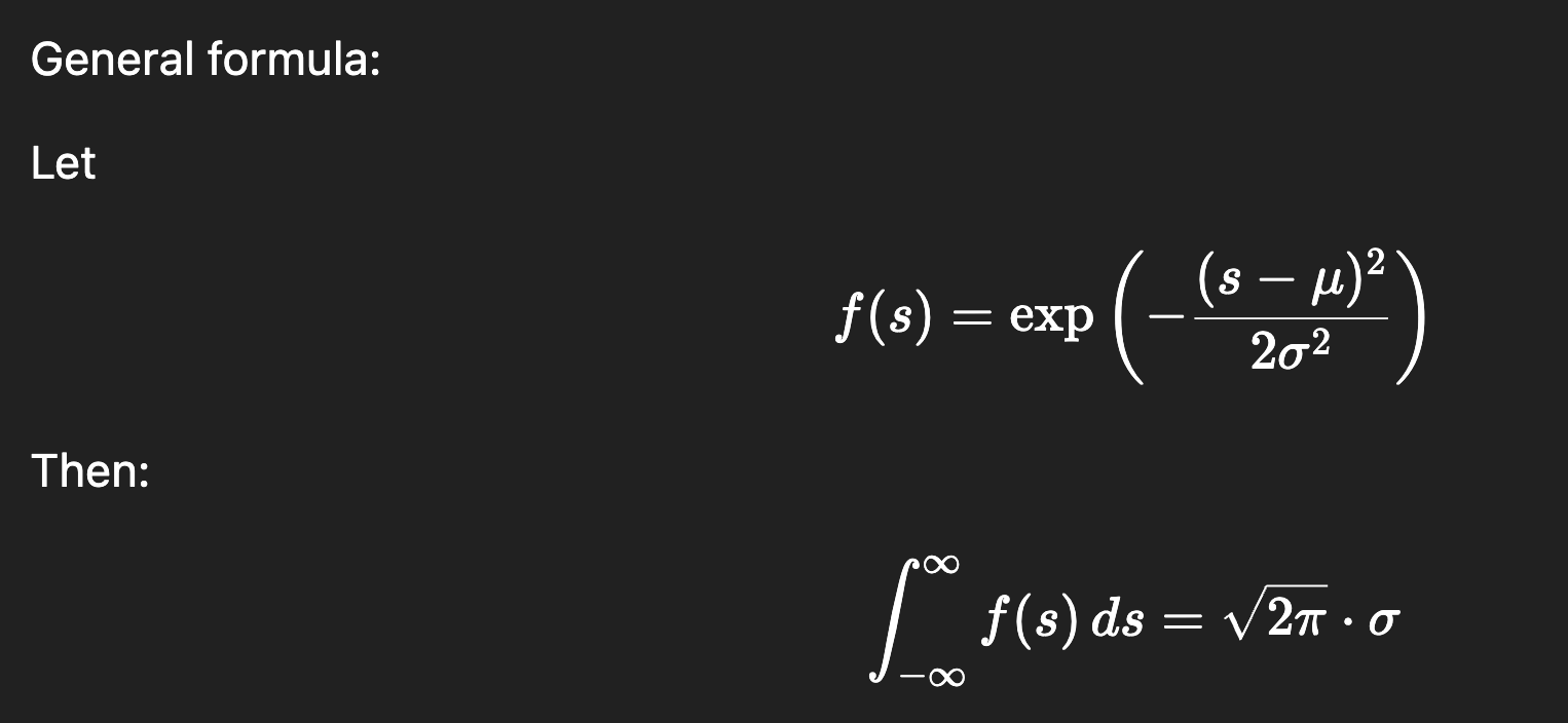
using standard gaussian integral

\[\int \exp\left( -\frac{A}{2} \left(s - \frac{B}{A}\right)^2 \right) ds= \sqrt{\frac{2\pi}{A}}\]

So final expression becomes:

\[\int \exp\left( -\frac{A}{2} \left(s - \frac{B}{A}\right)^2 \right) ds= \sqrt{\frac{2\pi}{A}}\] \[P(m_a, m_v | C=1) =\frac{1}{2\pi\sqrt{\sigma_{av,a}^2 \sigma_{av,v}^2+ \sigma_{av,a}^2 \sigma_p^2+ \sigma_{av,v}^2 \sigma_p^2}}\times\ \exp \left(- \frac{1}{2}\frac{(m_a - m_v)^2 \sigma_p^2+ (m_a - \mu_p)^2 \sigma_{av,v}^2+ (m_v - \mu_p)^2 \sigma_{av,a}^2}{\sigma_{av,a}^2\sigma_{av,v}^2 + \sigma_{av,a}^2\sigma_p^2 + \sigma_{av,v}^2\sigma_p^2}\right)\]

But in this experiment as we are using interleaved 2-IFC AV duration discrimination task we can ignore the prior in the model $\sigma_p^2\sim\infty$. Here are the reasons for why we can assume a flat prior for the dscrimination:

We are using interleaved 2-AFC task which the orrder is mixed.
In a single trial both the Standard and Test stimuli have the same properties, in other words noise

This simplifies the likelihood of common-cause to:

\[P(m_a, m_v \mid C = 1) = \frac{1}{\sqrt{2\pi(\sigma^2_{a} + \sigma^2_{v})}} \exp\left(-\frac{(m_a - m_v)^2}{2(\sigma^2_{a} + \sigma^2_{v})}\right)\]

💡 **Derivation from formulate with prior:** $$ P(m_a, m_v | C=1) =\frac{1}{2\pi\sqrt{\sigma_{av,a}^2 \sigma_{av,v}^2+ \sigma_{av,a}^2 \sigma_p^2+ \sigma_{av,v}^2 \sigma_p^2}}\times\ \exp \left(- \frac{1}{2}\frac{(m_a - m_v)^2 \sigma_p^2+ (m_a - \mu_p)^2 \sigma_{av,v}^2+ (m_v - \mu_p)^2 \sigma_{av,a}^2}{\sigma_{av,a}^2\sigma_{av,v}^2 + \sigma_{av,a}^2\sigma_p^2 + \sigma_{av,v}^2\sigma_p^2}\right) $$ In this equation lets assume $\sigma_p^2->\infty$ 1. Denominator the following term becomes: $$ \sigma_{av,a}^2\sigma_{av,v}^2 + \sigma_{av,a}^2\sigma_p^2 + \sigma_{av,v}^2\sigma_p^2 = \sigma_p^2(\sigma_{av,a}^2+\sigma_{av,v}^2)+\sigma_{av,a}^2\sigma_{av,v}^2\\ \sim \sigma_p^2(\sigma_{av,a}^2+\sigma_{av,v}^2) $$ we ignore the $\sigma_a^2\sigma_v^2$ part as it wouldnt be comparable 1. Numerator in Let’s isolate the dominant term when: $$ 𝜎_p^2→ ∞ $$ Then Only the **first term** grows without bound: $$ (m_a - m_v)^2 \sigma_p^2 $$ So the **dominant contribution** to the exponent becomes: $$ \exp \left( -\frac{1}{2} \cdot \frac{(m_a - m_v)^2 \sigma_p^2}{\sigma_p^2(\sigma_a^2 + \sigma_v^2)} \right) = \exp \left( -\frac{(m_a - m_v)^2}{2(\sigma_a^2 + \sigma_v^2)} \right) $$ 2. When we combine all: $$ P(m_a, m_v | C=1) \approx \frac{1}{2\pi\sigma_p\sqrt{\sigma_a^2 + \sigma_v^2}} \cdot \exp \left( -\frac{(m_a - m_v)^2}{2(\sigma_a^2 + \sigma_v^2)} \right) $$ 4. Then we renormalize: In general we can say that $$ \int exp[-\frac{1}{2}\frac{x^2}{A^2}]=\sqrt{2\pi} A $$ Here sicnce below equation integrates to unity. This amounts to **dividing by its own integral**: and $$ x=m_a-m_v\\ A=\sigma_{av,a}^2+\sigma_{av,v}^2\\ $$ $$ \int_{-\infty}^{\infty} \exp\left[-\frac{(m_a - m_v)^2}{2(\sigma_a^2 + \sigma_v^2)}\right] d(m_a - m_v) = \sqrt{2\pi(\sigma_a^2 + \sigma_v^2)}. $$ 1. Hence the correctly normalised, “flat–prior” likelihood is $$ P(m_a, m_v \mid C = 1) = \frac{1}{\sqrt{2\pi(\sigma^2_{a} + \sigma^2_{v})}} \exp\left(-\frac{(m_a - m_v)^2}{2(\sigma^2_{a} + \sigma^2_{v})}\right) $$

So that integration was used twice:

once to marginalise over sss,
once more (conceptually) to compute the normalising constant of the Δ\DeltaΔ-Gaussian.

Likelihood of independent sources (C=2):

\[P(m_a, m_v | C=2,s_a,s_v) = P(m_a) \cdot P(m_v)\] \[= \frac{1}{2\pi \sigma_{av,a} \sigma_{av,v}}\exp\left( -\frac{(m_a - s_a)^2}{2\sigma_{av,a}^2} -\frac{(m_v - s_v)^2}{2\sigma_{av,v}^2}\right)\]

Decision:

Finally model should compare the estimated duration for both ‘test’ and ‘standard’ intervals decision should be computed as:

decision should be computed as:

\[⁍\] \[P(\text{"test longer"}) = \Phi\left(\frac{D}{\sqrt{2}\sigma_{CI}}\right)\]

$\hat S_{CI,t}$ The final internal estimate for the duration of the test interval and $\hat S_{CI,s}$ is the final internal estimate for the standard interval after causal inference.

$\sigma_{CI}$ is the effective sensory noise (standard deviation) associated with the internal estimate in the causal inference model.